Tag: hacks
-

Neon Scope
It’s so hard for me to clean up my office. I’ll see a random collection of objects that I’m supposed to be sorting, putting away, and/or throwing in the garbage.. and I can’t help playing with them instead. This time the objects in question were an old CCFL backlight inverter, a neon flicker-flame bulb, and…
-
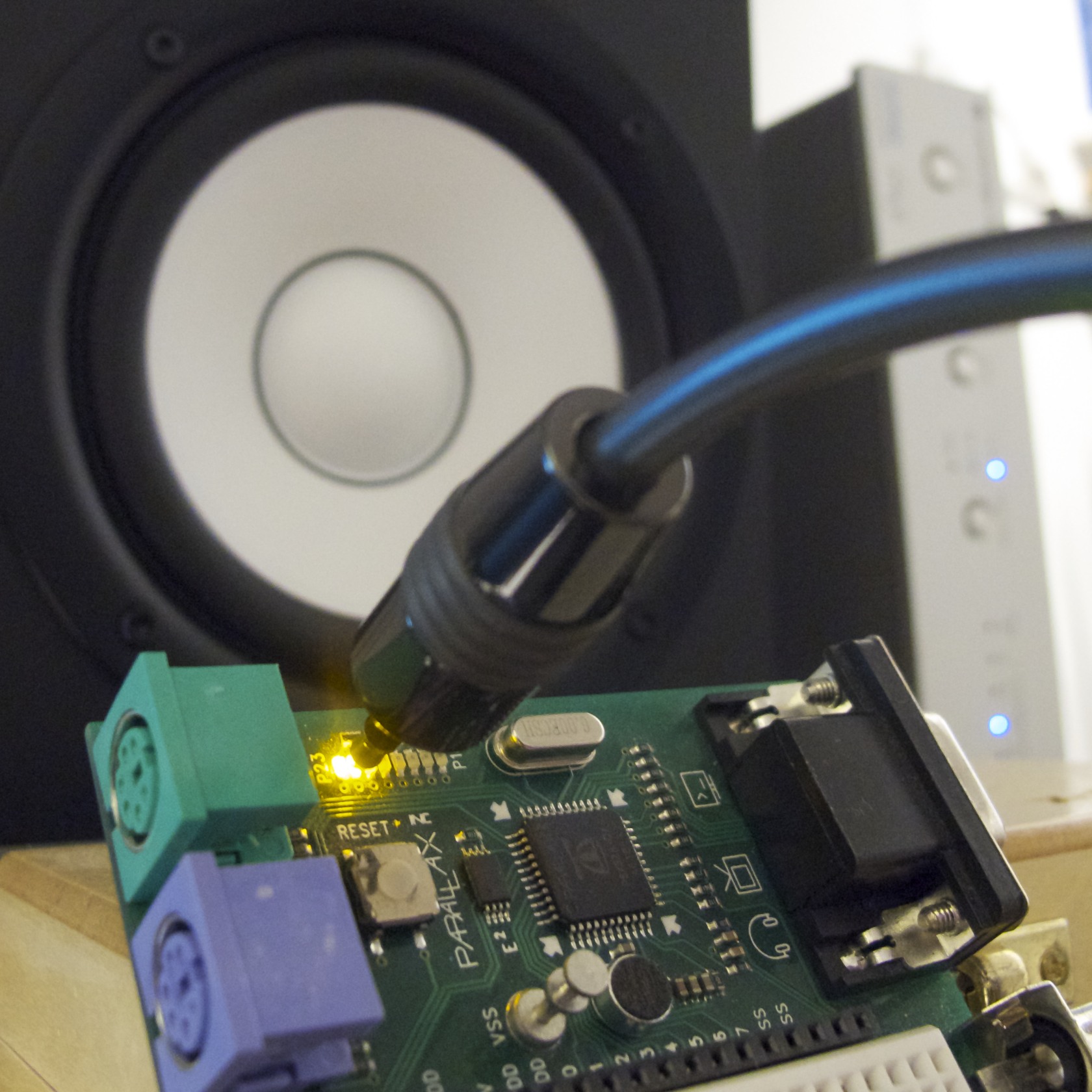
S/PDIF Digital Audio on a Microcontroller
A few years ago, I implemented an S/PDIF encoder object for the Parallax Propeller. When I first wrote this object, I wrote only a very terse blog post on the subject. I rather like the simplicity and effectiveness of this project, so I thought I’d write a more detailed explanation for anyone who’s curious about…
-

Hacking a Digital Bathroom Scale
People all around the internet have been doing cool things with the Wii peripherals lately, including the Wii Fit balance board. Things like controlling robots or playing World of Warcraft. But what if you just want one weight sensor, not four? The balance board starts to look kind of pricey, and who wants to deal…
-
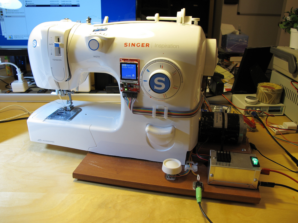
DIY Sewing Machine Retrofit
The story behind this project is a bit overcomplicated. That’s all below, if you’re interested. I made a video to explain the final product: Back Story This all started when I bought a sewing machine for making fabric RFID tags a little over a year ago, and started using it to make cute plushy objects.…
-
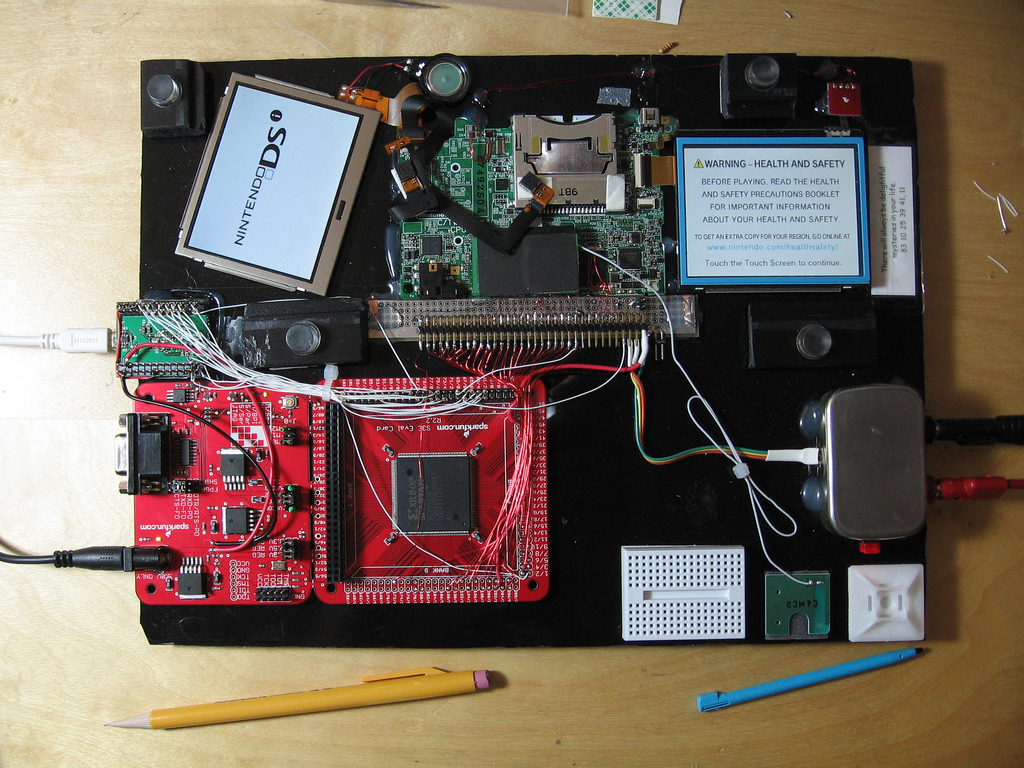
DSi RAM tracing
It seems like a lot of people have been seeing my Flickr photostream and wondering what I must be up to- especially after my photos got linked on hackaday and reddit. Well, I’ve been meaning to write a detailed blog post explaining it all- but I keep running out of time. So I guess a…
-
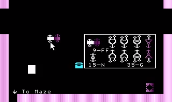
Robot Odyssey Mouse Hack 1
Yesterday I spent some more time reverse engineering Robot Odyssey. This was a great game, and it’s kind of a nostalgic pleasure for me to read and figure out all of this old 16-bit assembly. So far I’ve reverse engineered nearly all of the drawing code, big chunks of the world file format, and most…
-

A Binary Patch for Robot Odyssey
Robot Odyssey is one of the games that I have the fondest childhood memories of. It’s both a high-quality educational game, and a gentle (but very challenging) introduction to digital logic. There’s a Wikipedia article on the game. There’s also DroidQuest which is a Java-based clone of Robot Odyssey. The DroidQuest site also contains some…
-
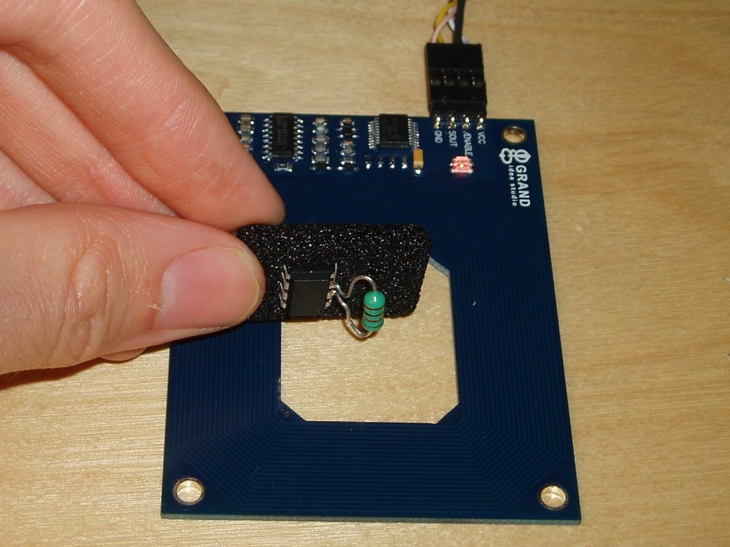
Using an AVR as an RFID tag
Experiments in RFID, continued… Last time, I posted an ultra-simple “from scratch” RFID reader, which uses no application-specific components: just a Propeller microcontroller and a few passive components. This time, I tried the opposite: building an RFID tag using no application-specific parts. Well, my solution is full of dirty tricks, but the results aren’t half…
-
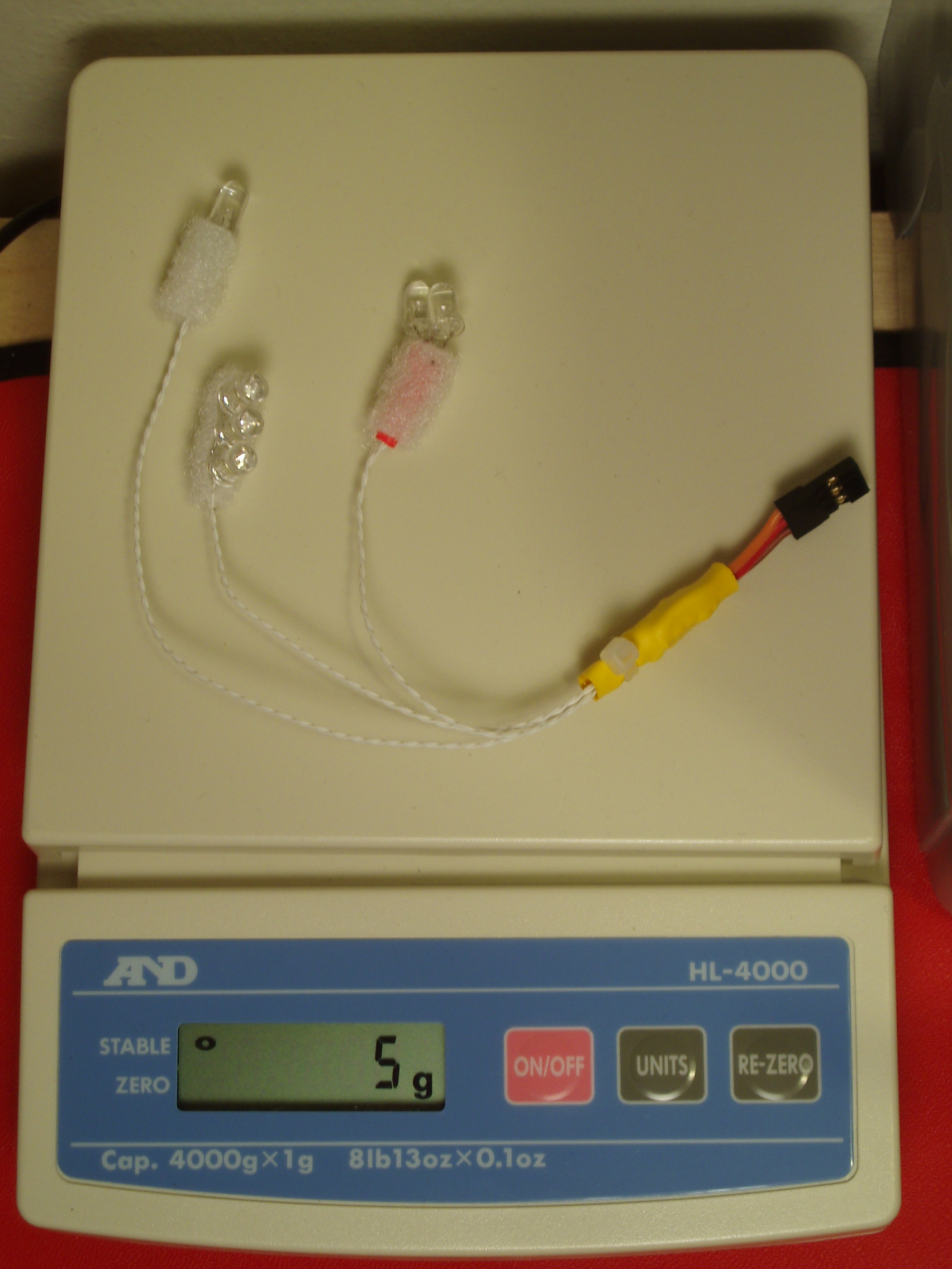
R/C helicopter lights, Revision A.5
Atmel is going to personally revoke my electrical engineering license if they ever find out what’s in that yellow heat-shrink blob, but I now have a shiny new 5 gram version of my helicopter light kit =D This version has all the same remote-control dimming and strobe capabilities of the heavier Revision A. The only…
-

Flightaware route histogram
Flightaware + Fyre: The above image is part of a histogram generated from Flightaware’s 24-hour time lapse. Click the link for the uncropped version. The original video is a Quicktime wrapper around individual PNG frames. I used mencoder to strip off the Quicktime wrapper, then a small Python script split the video streams into individual…